In “Rows and Columns, Part 1: Jump-starting Analysis Using Spreadsheets,” I revealed the magic of using filtering, drop-down menus, and checkboxes in analyzing your user-research projects. Now in Part 2, I’ll discuss how you can use formulas to make your analyses easier to understand. If you’re new to using spreadsheets, you might find formulas somewhat intimidating. Some of them tend not to be very intuitive.
In Part 2, I’ll continue using the fictional example that I used in Part 1, which focuses on the Vinyl Exchange, a digital marketplace for buying and selling music.
Champion Advertisement
Continue Reading…
Comparing the COUNTA and COUNT Formulas
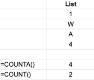
What do you think COUNTA() does? (If you think it counts the number of A’s in your spreadsheet, you’re wrong!) COUNTA() actually counts a number of items, while COUNT() counts a number of numbers, as shown Figure 1. A field that contains both numbers and strings could benefit from COUNTA.
Figure 1—COUNTA and COUNT formulas
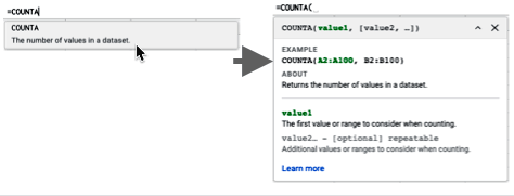
However, if you’re not sure what a formula does, you can always look up its definition within your spreadsheet application, simply by typing an equals (=) sign and the formula into the formula-entry area, then selecting a formula suggestion, as Figure 2 shows.
Figure 2—Formula Help
Now, let’s begin our exploration of some formulas that you’ll find particularly useful for your UX research projects.
COUNTIF() Formula
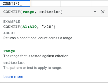
COUNTIF() is a formula that lets you calculate subtotals within a list. It takes two parameters: a range of cells that include values and a set of conditions, or criteria, that a formula must satisfy to increment the count. Figure 3 shows an example.
Figure 3—COUNTIF() formula
When you need to present a subset of your data in a table format, COUNTIF() is a good choice.
COUNTIF() Formula Example
When it’s time for a readout of your research findings, one big question stakeholders often ask is: “To whom did you speak?” Stakeholders want to make sure that you’ve interviewed the right people for your study. It’s important to show stakeholders who has participated in your research. This makes your stakeholders more confident in your findings, in addition to making your findings more meaningful and valid for decision-making.
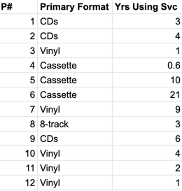
Part of ensuring that you’ve spoken with the actual target users is collecting data on the common attributes of people in that group. An efficient way of tallying up various attributes of your participants is through the use of the COUNTIF() function. For example, if you did a study with Vinyl Exchange users and were interested in tallying up some data about your participants, your stakeholders might ask about the participants’ level of experience with the Web site or what music formats the company primarily sells on the site. Figure 4 shows the data you would need to tally.
Figure 4—Data to tally
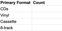
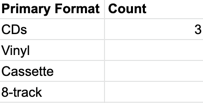
Set up a table within the same worksheet as the data so you can quickly refer back to the original data in case there is an issue with the formula. Do this by adding two columns: one for the primary data you are tallying—for example, the Primary Format—and another column for the counts—for example, Count, as you can see in Figure 5. Once you’ve created your column headers, enter all of the possible values in the first column, as Figure 5 shows. The primary formats would be CDs, Vinyl, Cassette, and 8-track. Make sure that the values in your spreadsheet exactly match those in your data, including their case. Otherwise, you may end up with miscounts when you add up your formulas. If your data is a bit sloppy, you should go back and sanitize it so the data is completely consistent.
Figure 5—Adding the values to tally to your table
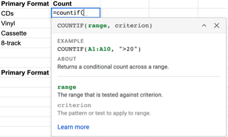
Once all the values that you’ve entered are in the right case, it’s time to begin entering the formulas. Starting with the first cell under Counts, type =COUNTIF(. You’ll notice that, as you start typing the formula, a contextual Help pop-up provides the correct syntax for inputting the parameters into the formula, as Figure 6 shows.
Figure 6—Typing a COUNTIF() formula
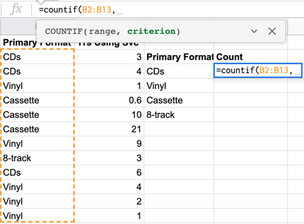
For the first parameter, range, select the entire column of items that you’re tallying. But you shouldn’t select the column header or the entire table. Just select the Primary Format column’s data, as shown in Figure 7.
Figure 7—Selecting a range of items for the COUNTIF() formula
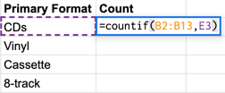
The next parameter you’ll need to include is the criterion, which is the filter you’ll apply to the selected range. The quickest way to tally up the count for every primary format is by referring to the value in the first column. Rather than your explicitly typing the value CDs, your formula can refer to the value in that first cell—whatever it is—as shown in Figure 8.
Figure 8—Referring to the first column for the criterion parameter
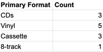
Once you’ve added the criterion and ended the formula with a closing parenthesis, press ENTER. The cell value updates to the count for the respective item in the first column, as shown in Figure 9.
Figure 9—COUNTIF() with both parameters in first row of the table
Remember to Lock the Range
If you’re unfamiliar with the way spreadsheets work, you might assume that you can simply copy and paste the contents of the cell containing the formula into the remaining cells in the Count column. However, if you did that, you would get some funny results—even though everything would appear fine at first glance, as Figure 10 shows.
Figure 10—Pasting COUNTIF() into remaining cells of Count column
Although the spreadsheet won’t generate an error, if you took a closer look at the data table that is shown in Figure 4 and reviewed the counts for vinyl, would they be correct? Technically, yes. There are five participants who primarily sell vinyl in the main data table. Look at the range values in the count for CDs. The range parameter in the initial cell for Count was B2:B13. That range defines the complete list of items to be filtered. When you copied the formula and pasted it into the Count cell for vinyl, it incremented the numbers to B3:B14. Although B14 is actually a blank cell, in this case, even though the range is off, the number is still correct.
To preserve, or lock, the range B2:B13 each time you copy and paste the formula, you need to add a $ preceding each letter and number, as follows: $B$2:$B$13.
Now, once you’ve entered the formula into the first cell of the Count column, copy and paste it into the remaining cells of that column. You should see the same result as in Figure 10—except your formula would now be correct.
COUNTIF() for Tallying the Frequency of Findings
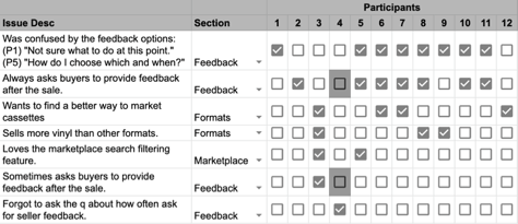
Aside from aggregating participant metrics, COUNTIF() is a great formula for tallying how frequently a particular finding occurs in your research findings. Let’s say that you needed to keep track of how often participants became confused by the feedback options that you presented to them in your findings spreadsheet for UX research involving the Vinyl Exchange feedback workflow. In addition to this finding, you also logged some other potential themes during your analysis, as Figure 11 shows.
Figure 11—Spreadsheet for gathering your findings
Let’s add a column called Frequency to the next available cell. Then insert the COUNTIF() formula in that cell to keep track of how often various issues occurred. In the first cell, enter =COUNTIF(E3:P3,TRUE). The first parameter in the formula is the range of participants, each of which appears in the form of a checkbox. (For more information about adding checkboxes to your spreadsheets, check out my previous column, “Rows and Columns, Part 1: Jump-starting Analysis Using Spreadsheets.”) The second parameter is the criterion that must be satisfied for the formula to increment the count. Because the value of a checkbox can be only TRUE, or checked, or FALSE, or unchecked and we want to count only participants for whom there was a particular finding, we can define that second parameter as TRUE.
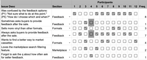
Because you’re counting the instances in each row, you don’t need to lock the range with $ signs. The range should increment when you copy and paste it into the remaining cells in the Frequency column. Once you’ve copied and pasted the formula into the remaining cells, you should see the frequencies shown in Figure 12.
Figure 12—Findings with frequencies using the COUNTIF() formula
Sorting Frequencies
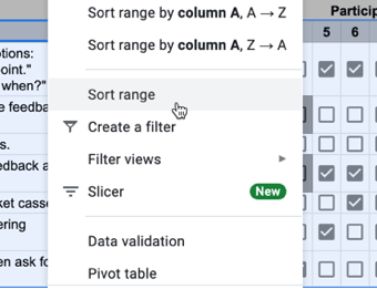
The real value of using the COUNTIF() formula within the context of your findings is that it lets you very quickly see which of your findings are most frequent and, therefore, are most likely to make it into your final research report. To see the most frequent findings, you must sort the Frequency column in descending order, so the most frequent findings appear at the top of the table. To do this, you must first select the entire table. Then, in the Data menu, choose Sort range, as shown in Figure 13.
Figure 13—Sort range menu option
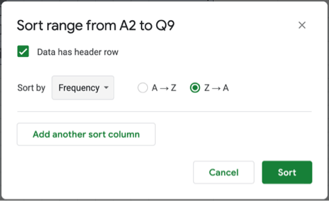
In the Sort range dialog box, shown in Figure 14, select the “Data has header row” checkbox, causing the columns from your selected table to populate the column picker. In the Sort by drop-down list, select Frequency, then select the Z → A option to sort the column in descending order. Then click the Sort button
Figure 14—Sort range dialog box with Sort by: Frequency selected
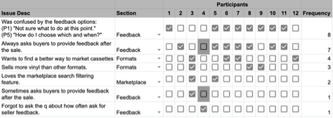
As shown in Figure 15, you should now see the counts in the Frequency column in descending order.
Figure 15—Findings table with Frequency counts in descending order
As you proceed with your analysis and the frequency counts update, you must refresh the sort, as I’ve just described, because the spreadsheet won’t automatically update it for you. I recommend refreshing the sort again after analyzing a large amount of data or even waiting to sort until you’ve finished tallying all of your data.
Next in My Rows and Columns Series
In Part 3 of my “Rows and Columns” series, I’ll explain how to spice up your spreadsheets with conditional formatting, which lets you visualize themes in your data more easily.
Michael has worked in the field of IT (Information Technology) for more than 20 years—as an engineer, business analyst, and, for the last ten years, as a UX researcher. He has written on UX topics such as research methodology, UX strategy, and innovation for industry publications that include UXmatters, UX Mastery, Boxes and Arrows, UX Planet, and UX Collective. In Discovery, his quarterly column on UXmatters, Michael writes about the insights that derive from formative UX-research studies. He has a B.A. in Creative Writing from Binghamton University, an M.B.A. in Finance and Strategy from NYU Stern, and an M.S. in Human-Computer Interaction from Iowa State University. Read More